An introduction to algorithm complexity analysis (I)

I cannot understand how many problems a lot of students have in learning the principles of algorithm complexity. So, finally, I have decided to prepare a short introduction and some tricks in order to help them.

In a previous post, I described some of the strong points in order to take into account the complexity analysis before coding. In this post I'm going to describe the four basic steps you must follow in order to study the complexity of an algorithm. In future posts, I will provide more details and examples for each step.

The first thing to take into account is the difference between efficiency and effectiveness. Effectiveness means that the algorithm carries out its function, it is correct. But when we talk about efficiency, we are looking for something else ... we want a correct algorithm and with the best performance.

Basic steps in complexity analysis of an algorithm

1. Select the computational resource you want to measure. Normally we have two options: time and memory. But other studies can be undertaken like, e.g., network traffic.

2. Look to the algorithm and pay attention to loops or recursion. Try to see the variables and conditions that makes the algorithm to work more or less. Sometimes is one variable, some times several ... This is going to be our size of input. Remember that with complexity analysis we are interested in getting a function that relates the size of input with the computational resource.

3. Once we have the size of input of the algorithm, try to see if there are different cases inside it. Normally we have to pay attention to the best, worst and average cases. What are 'cases' in this context ? Circumstances in which the algorithm can work differently. These cases NEVER depends on specific values (high or low) of the size of input. NEVER. To work with an array of 1 million components is not a 'worst case', is just a specific size of input which is going to have a resulted time or memory consumption.

To have different cases means that you are not able to provide just one function that relates the size of input with the computational resource. Probably, having for example a worst and best cases means that you are going to have two different algorithm behaviours. It is like having two algorithms inside the algorithm.

So, in the definition of the different cases you are not allowed to use the term 'size of input'. It has to be another thing. Look the loops or recursion, and try to see specific conditions that make the loop or recursion to finish before scheduled, before the end of the input range. Normally, there you have the clue of different cases. An example ? The linear search of an element inside an array. In such a case, if the element we want to look for is not inside the array, the algorithm, in order to provide a negative answer, has to go from the beginning to the end of the array. That's the worst case. But if the element we want to look for is in the first position of the array, then there is no iteration. We find the element immediately. That's the best case. Note that the 'size of input' of this algorithm, the number of elements of the array, is not part of the definition of best and worst cases.

Take into account that it is not only important to detect these cases, but to be able to define them, to describe in which circumstances we are in front of each case.

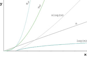
4. Now, for each of the cases our algorithm has, we have to count computational resource consumption. If we are studying temporal cost, for example, then we have to count instructions (or calls in a recursive algorithm). What we need is the function which relates the size of input with the computational resource. And in this function we are interested in its highest degree, i.e., we are interested in its asymptotic profile (how the algorithm works for high values of the size of input). At the end of this step, the important thing, rather than follow a correct notation, is to be able to show if the algorithm, and for each case, is LINEAR, QUADRATIC, EXPONENTIAL, LOGARITHMIC, etc.

These are the basic steps to follow in order to face the algorithm complexity analysis. In future posts, I will try to provide more details for each of these steps and some examples.